Kristin Kinic, MS
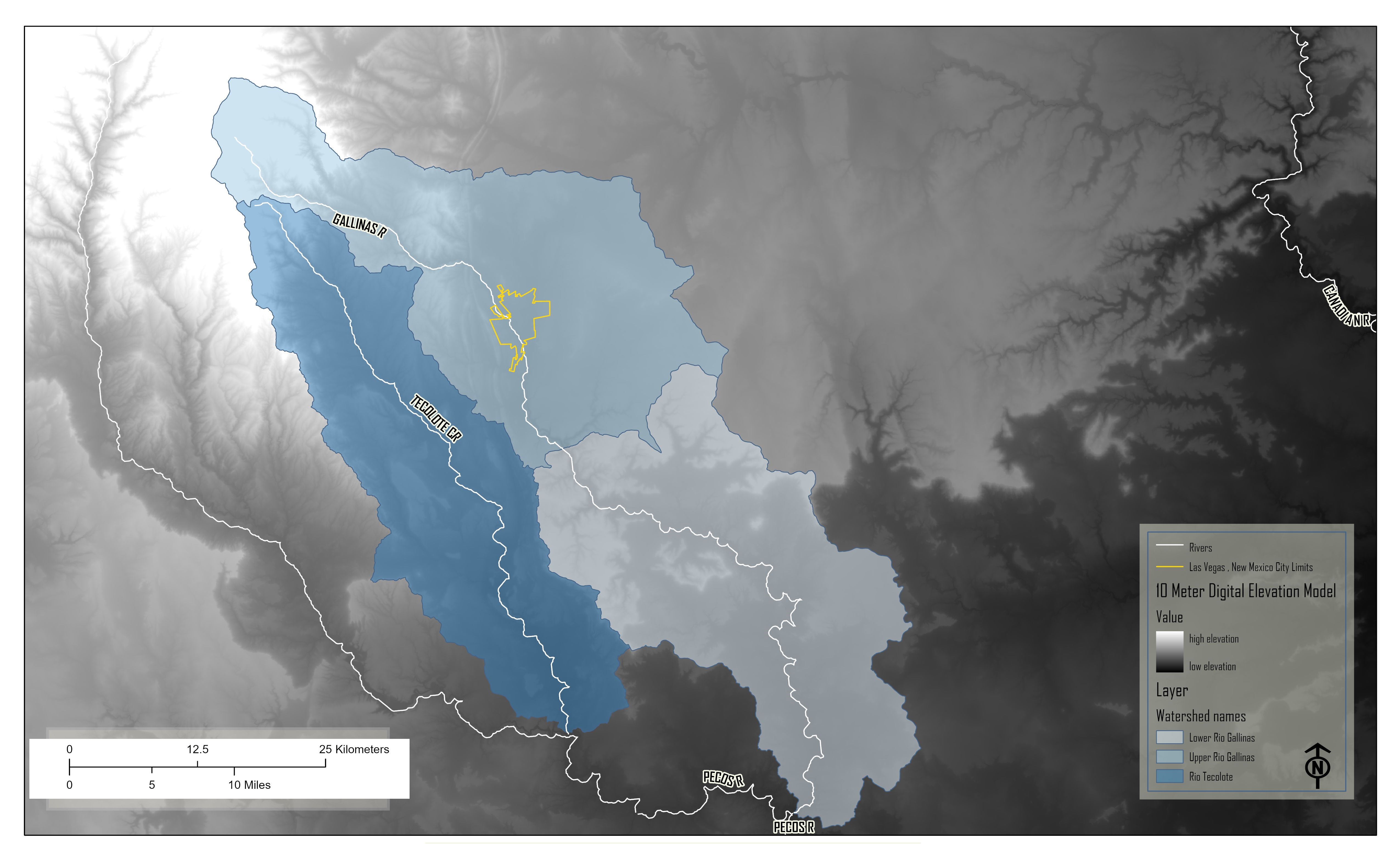
Inspiration to study Hydrologic Processes in Las Vegas, New Mexico
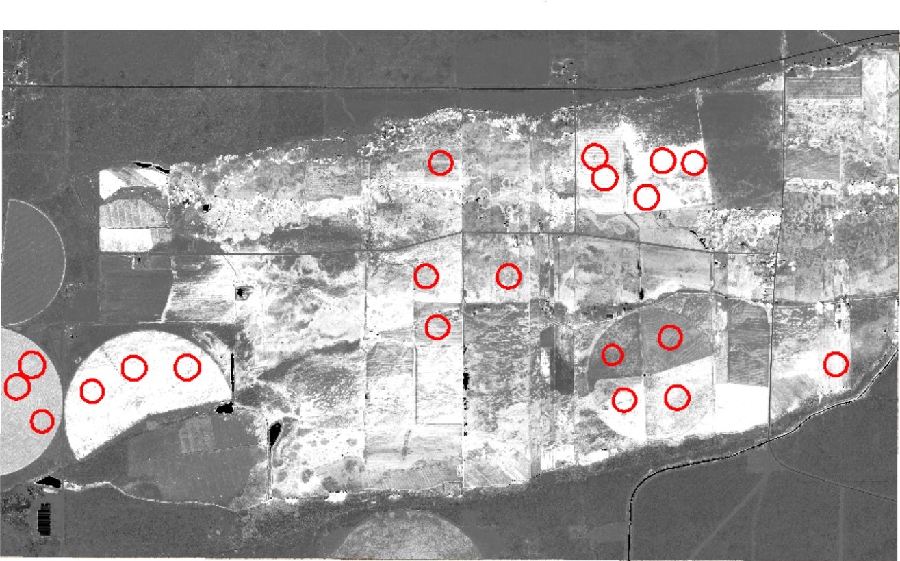
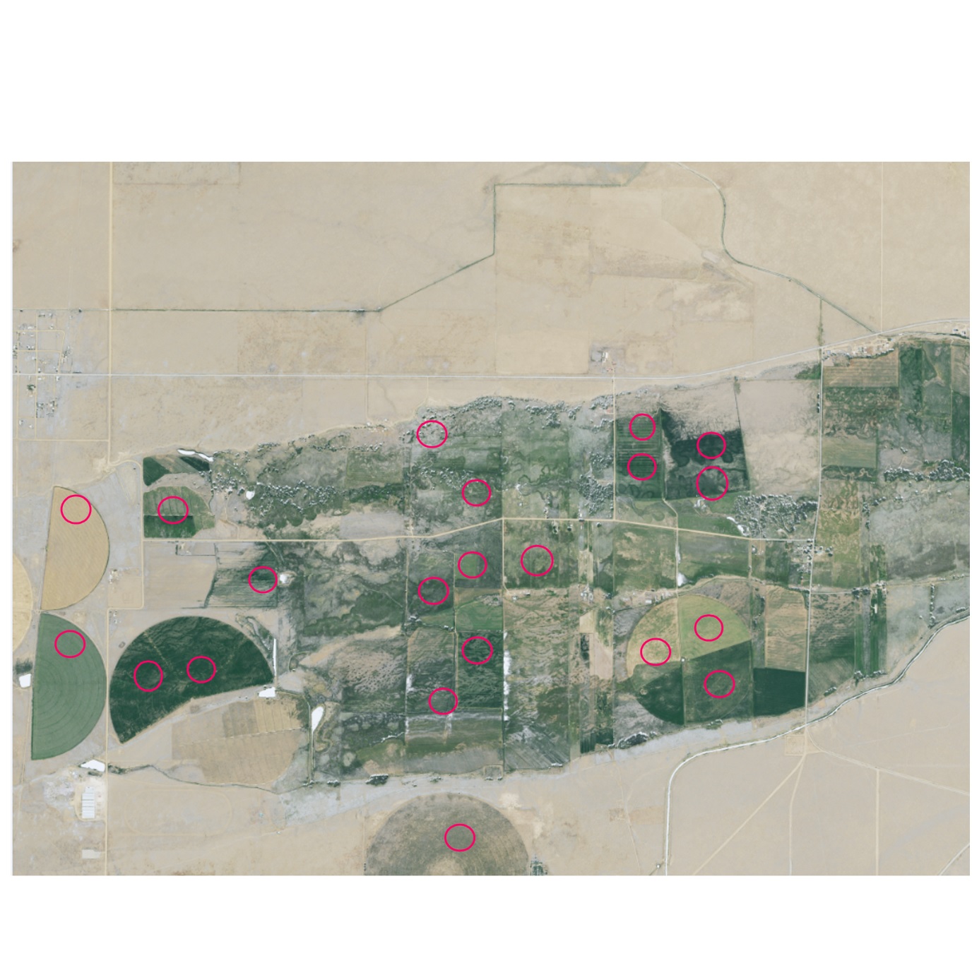
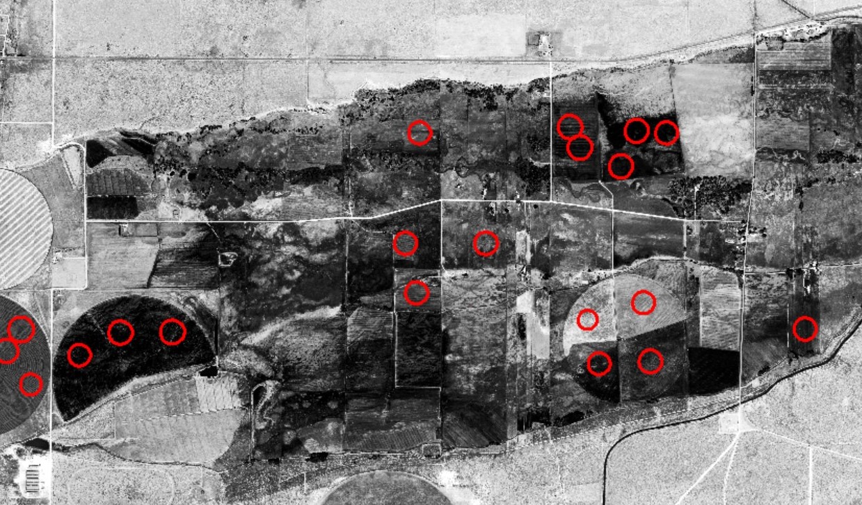
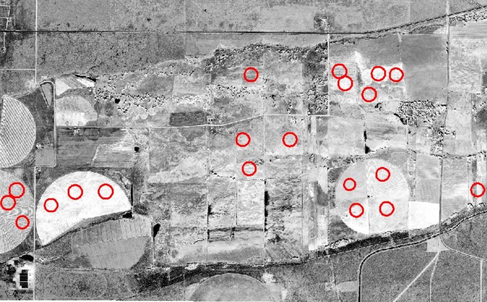
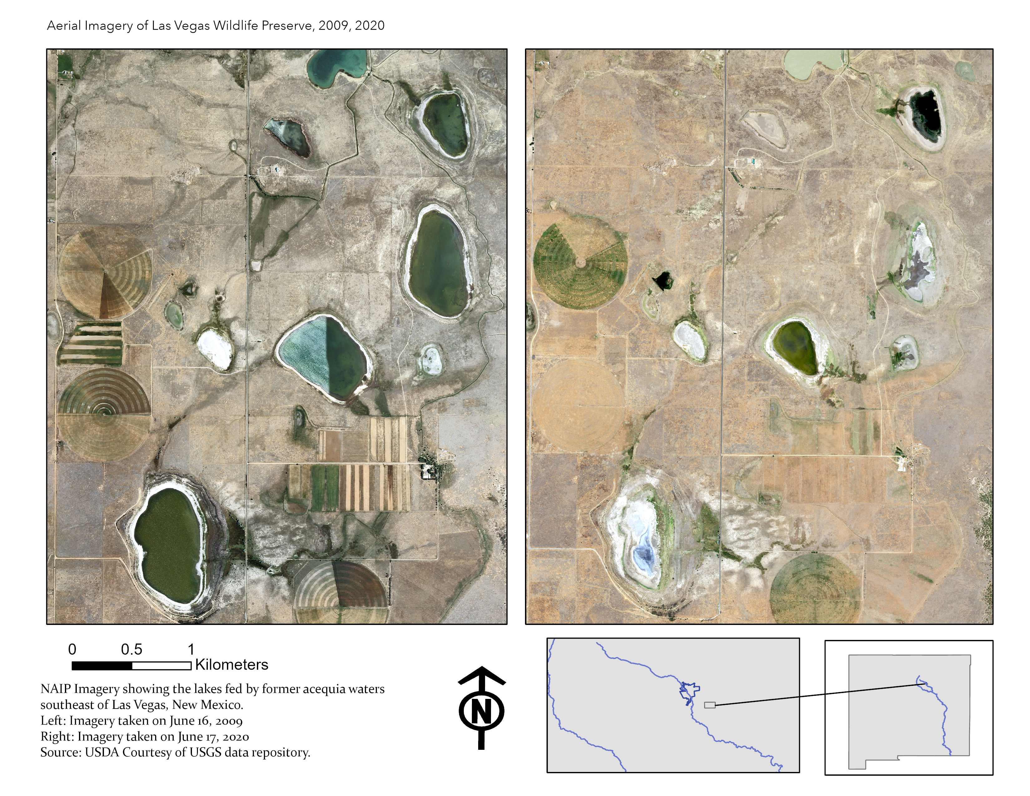
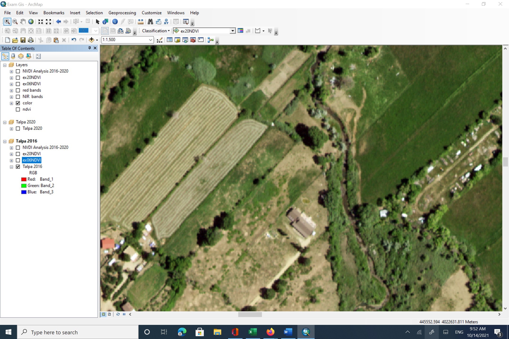
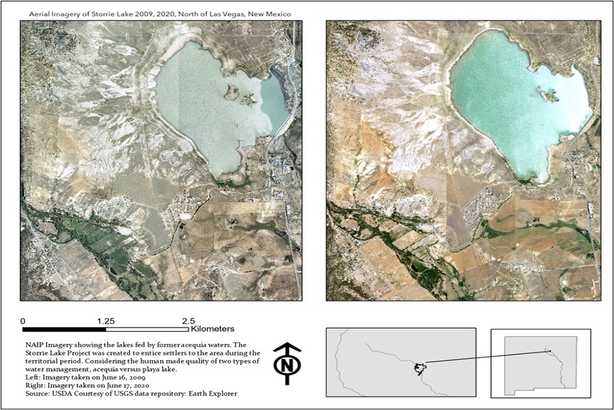
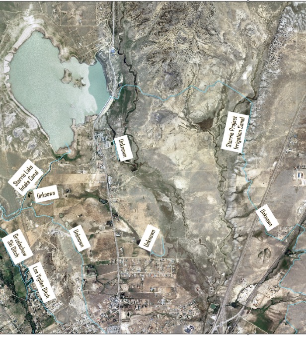
The Las Vegas area has several water impoundments, some healthy acequias, remnant acequias. These NAIP images show two different water management tactics: Storrie Lake and the Middle Gallinas Acequias.
Superscript
What is NDVI (red)
NDVI: Natural Vegetation Difference Index
NDVI has a fixed scale, from 1 to -1. NDVI is
calculated by isolating elements of electromagnetic spectrum inherent in aerial and satellite imagery and then layering those elements to filter out "noise"
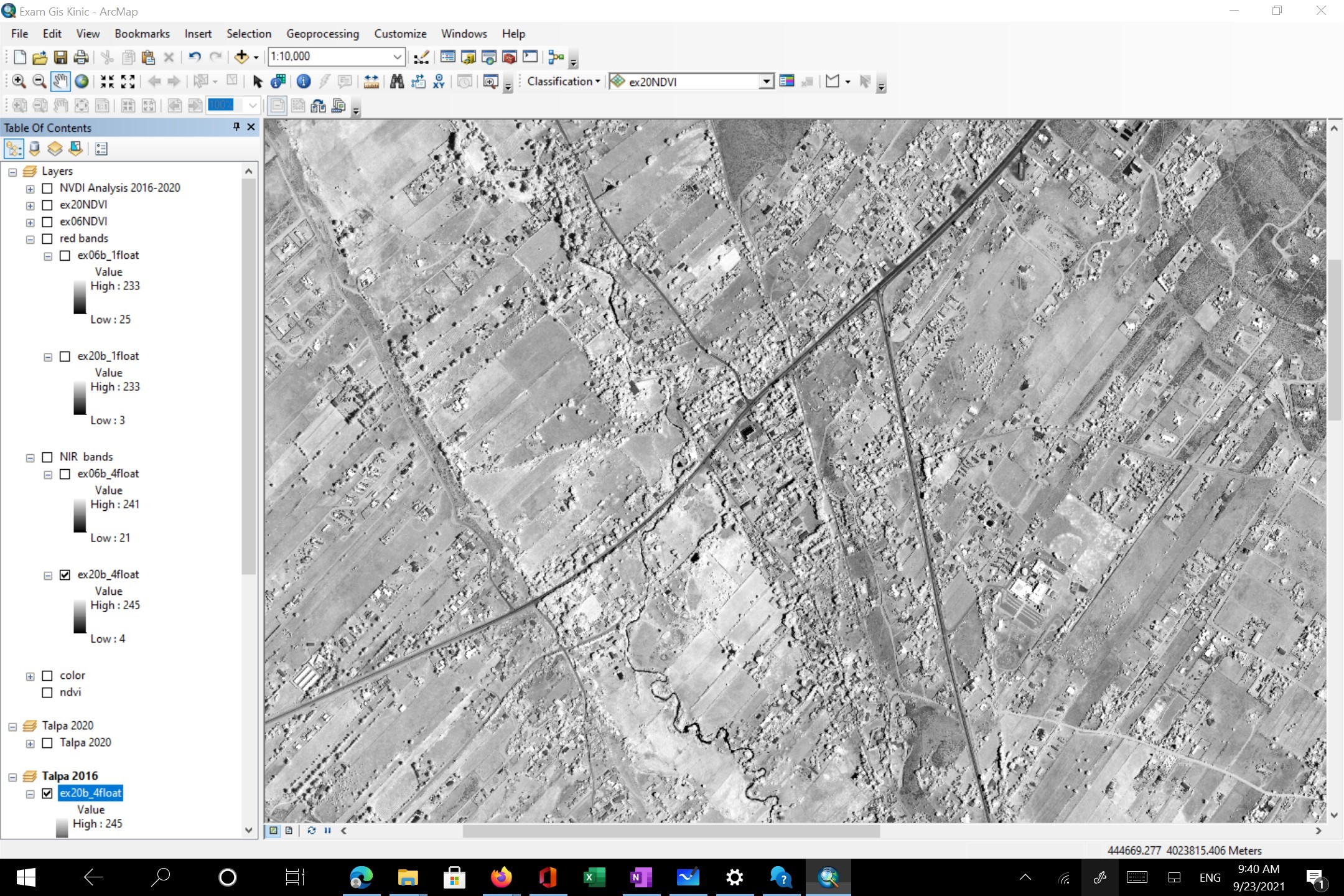
to better visually appreciate healthy vegetation. In NAIP imagery, there are 4 bands
readily available for this analysis, and I will be using two of them, in raster
form, band 1(red) and band 4 (near infra-red or NIR). The numerical value of
each raster will be used in this formula, NDVI(red)= NIR-RED/NIR+RED .
NDVI (red)
Statistical Hypotheses:
H/0 = µNDVI/ace = µNDVI/cpi
H/A = µNDVI/ace > µNDVI/cpi
H/A= Crops
that are watered by acequias or central pivot irrigation systems have different NDVI values.
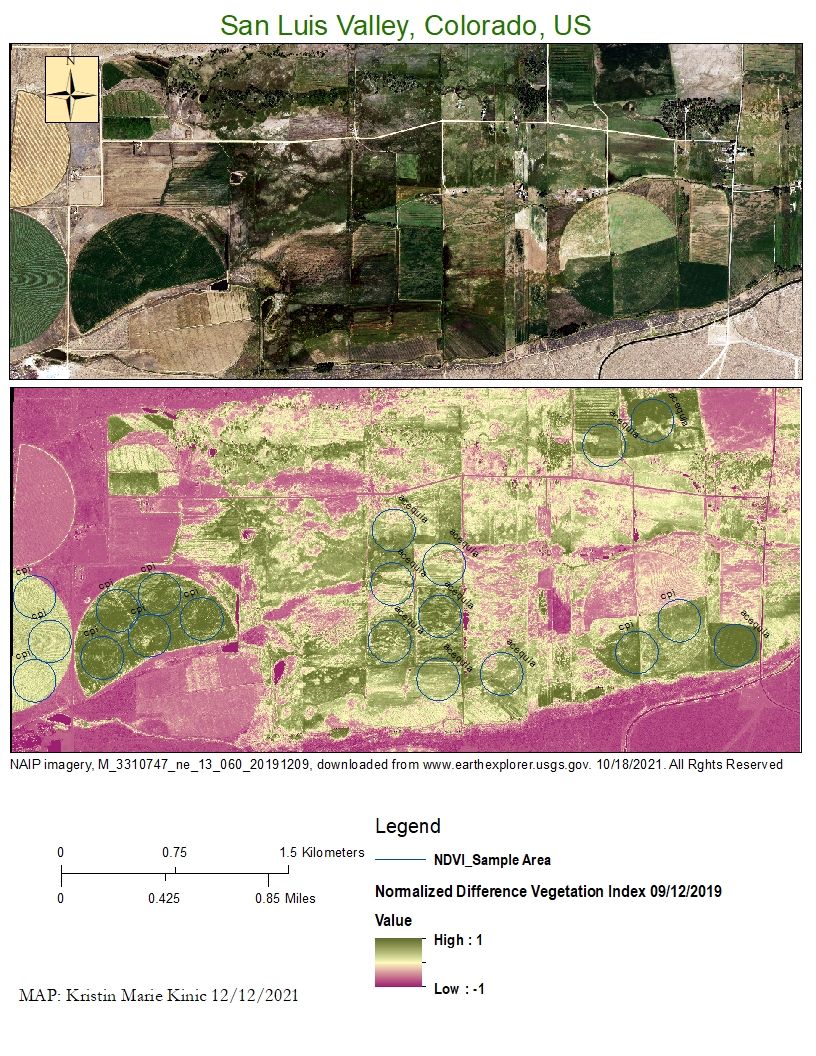
METHODS: Identified
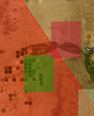
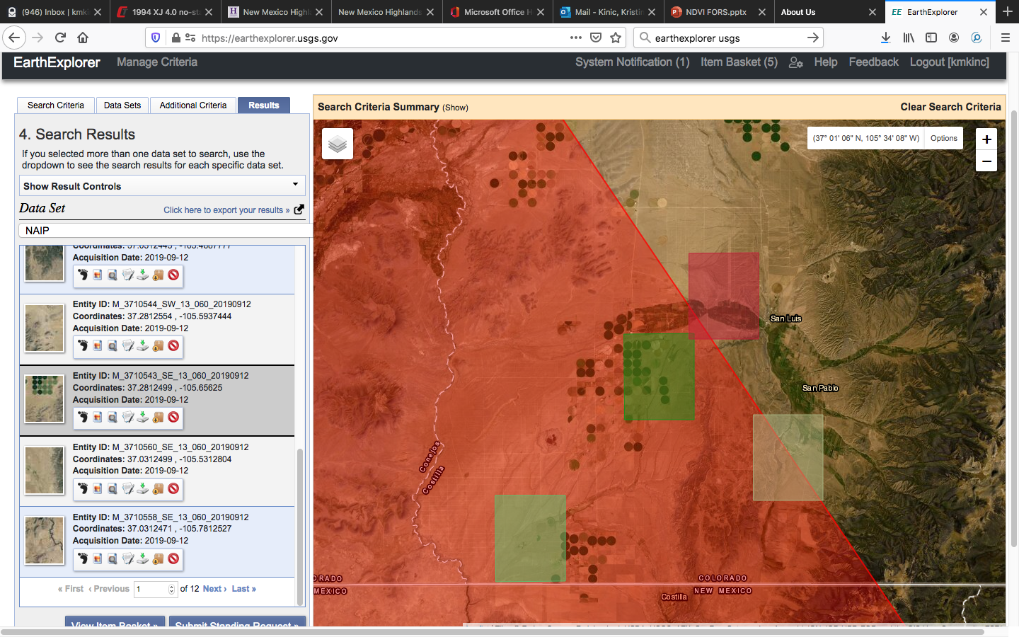
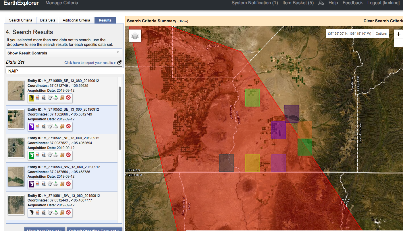
potential agricultural sites for NDVI analysis using NAIP aerial photography of agricultural areas in Southern Colorado and Northern New Mexico. I will use
remote sensing to find n= 20 study areas, with paired samples. The pairs will
consist of two types of agricultural sites: those with acequias and those with center
pivot irrigation. On site assessments of acequia ditches will be conducted to
establish appropriate acequia samples, to inventory beneficial,
non-cultigen flora. Examples of beneficial flora are red willow, and seges. Water
temperatures in ditches will also be taken for future research. To
ensure rigor, I will randomize sample points in circular plots with radii of
200m, in Arc Map ™. I will then use these points to calculate NDVI to describe
the health and prosperity of cultigens on the ground of both types of irrigation: acequia and pivot
irrigation. NDVI has a fixed scale, 1 to -1. NDVI is calculated by isolating
elements of electromagnetic spectrum inherent in imagery and then layering
those elements to filter out "noise"
to better appreciate healthy vegetation. In NAIP imagery, there are 4 bands
readily available for this analysis, and I will be using two of them, in raster
form, band 1(red) and band 4 (near infra-red or NIR). The numerical value of
each raster will be used in this formula, NDVI= NIR-RED/NIR+RED.
Steps leading to statistical Analysis using RStudio
create uniform areas that are >4500<5000m^2
separate raster data into bands in Arc Map
compute NDVI in Arc Map
create random samples in the areas in ArcMap
collect numerical data
save numerical data in .csv format
import .csv into R Studio
Use procedural flowchart to select a test
test assumptions of that test
test normality of data and homogeneity of variance
run tests to either a. reject the null hypothesis and b. accept the the alternate hypothesis.

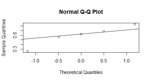
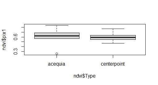
R outputs (below) show some of the process of the statistical analysis. On the left, is one of the 6 theoretical quantile plots I used to visually assess the data. This one is the assessment of the normality of the data from an average of NDVI points from the acequia study areas in the sample part called pixel 1. I sampled each site 3 times, the data sets were named pixel 1, pixel 2, pixel 3. While there are probably better way top sample in NDVI. I used the Pixel Inspector tool that gives the value of pixels in a tabular data frame. I simple entered the first three columns of point (pix 1,2,and 3 in the code) into a csv file, for n=10 sites. In total I had 900 points, n=10(30x3). The points were then averaged. For this analysis I used the type of irrigation (acequia, and center point) as my predictor or independent variable and the NDVI value (a continuous numerical value from 1, to -1) as the response or dependent variable.
Results of the Shapiro Wilkes tests and Fligner tests showed that all of the data was normally distributed with significant p value >0.05. In addition, Fligner tests showed that all of the variances in the data sets were homogeneous. I then conducted a two sample t test.
